General visualizations
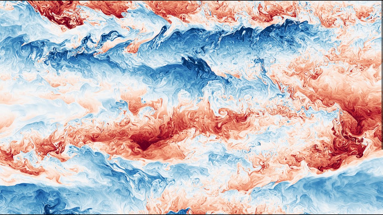
Forced no shear
Passive Scalars in Stratified Turbulence
1 — Scalar mixing layers in decaying homogeneous turbulence
This simulation is based on case III in de Bruyn Kops and Riley [2019]. The flow is initially homogeneous and isotropic in power-law decay. At dimensionless time \( t^* = 1 \), the density field is initialized to be a uniform gradient in the \(z\)-direction and stratified turbulence develops. Also at \( t^* = 1 \), three passive scalar fields are imposed. Two are scalar mixing layers that vary in the \(x\) and \(y\) directions, respectively, and the third is a narrow plume in the \(z\) direction. Movies of the passive scalars follow.
2 — Passive scalar in stationary homogeneous sheared stratified turbulence
This simulation is based on case R1 in Portwood et al. [2022]. The is shear and gravity is tuned so that the flow is quasi-stationary. In the current case, the active scalar has Prandtl number \( Pr=7\) and the passive scalar has \(Pr=50\). Both have the same stationary mean gradient. When the simulation starts, the velocity and density fields are in quasi-equilibrium and the passive scalar is identical to the density. At time advances, the smaller scales develop in the passive scalar. Movies of the density and passive scalar follows. The top panel shows the full \( xz\) slice of the scalar and the lower panels show the passive scalar and the density in a subset of the domain at full resolution.
3 — Passive plumes in stationary homogeneous sheared stratified turbulence
This simulation is based on case R1 in Portwood et al. [2022]. The is shear and gravity is tuned so that the flow is quasi-stationary. In the current case, the active scalar has Prandtl number \( Pr=7 \) and passive scalar plumes have \( Pr=50 \). The top panels shows the full \( xy \), \( xz \), and \( yz \) slices of the plumes, and the lower panels show subdomain. The location of the subdomains are outlined in white in the top panels.