Datasets
Datasets, and associated analysis tools and demos, will progressively be added to the tables below. Data are hosted on the Constellation repository and may be downloaded to a local computer using Globus. If you are interesting in exploring datasets not currently archived on Constellation, please contact the group.
General details about the simulations are provided within the collapsible headings below.
Equations of motion
All direct numerical simulations (DNS) are performed under the following conditions.
The density field $\rho$ satisfies \begin{equation} \rho\left(\mathbf{x},t\right)=\rho_{0}+\bar{\rho}\left(z\right)+\rho’\left(\mathbf{x},t\right),\ \ \bar{\rho}\left(z\right)=-Az, \end{equation} where $z$ is taken to point upward in the opposite direction of gravity, $\rho_0$ denotes a reference density, $A$ is a constant describing the linear background vertical density gradient, and $\rho’$ denotes (turbulent) fluctuations away from the background state.
The Navier-Stokes equations are then solved under the Boussinesq approximation; specifically, variations in density away from the background reference value $\rho_0$ are assumed to be small and such density variations are thus only accounted for when computing the buoyancy force. The resulting equations of motion that are solved numerically are:
\[\begin{align} \nabla\cdot\mathbf{u} &= 0, \\ \rho_{0}\left(\frac{\partial\mathbf{u}}{\partial t}+\left(\mathbf{u}\cdot\nabla\right)\mathbf{u}\right)&=-\nabla p'+\mu\nabla^{2}\mathbf{u}-\rho'g\hat{\mathbf{z}}+\mathbf{F}, \\ \frac{\partial\rho'}{\partial t}+\mathbf{u}\cdot\nabla\rho'+w\frac{\partial\bar{\rho}}{\partial z} &= \kappa\nabla^{2}\rho'. \end{align}\]Equation (2) is the incompressibility condition arising from mass conservation under the Boussinesq approximation, with $\mathbf{u}=\left(u,v,w\right)$ describing the fluid velocity. Equation (3) is the momentum equation, where the pressure field has been decomposed as $p\left(\mathbf{x},t\right)=\bar{p}\left(z\right)+p’\left(\mathbf{x},t\right)$ such that $\partial\bar{p}/\partial z=-\rho_{0}g$ (i.e. $\bar{p}\left(z\right)$ is the hydrostatic pressure arising from the ambient density $\rho_0$). The gravitational acceleration is $g$, the viscosity $\mu$, and $\mathbf{F}$ denotes a body force that is used in some simulations to sustain turbulence in a steady-state (i.e. statistically-stationary turbulence). Equation (4) is an advection-diffusion equation governing density perturbations $\rho’$ away from the linear background stratification, with $\kappa$ denoting the molecular diffusivity.
A fractional-step pseudospectral method is used to solve equations (2-4) in dimensional form in a three-dimensional box. The variables $\mathbf{u}=\left(u,v,w\right)$ and $\rho’$ all satisfy periodic boundary conditions. Values of the following constants are provided with each dataset in a text file “params.txt”:
| $L_x, L_y, L_z$ | Box dimensions |
| $N_x, N_y, N_z$ | Number of grid points in each dimension |
| $g=1$ | Gravitational acceleration (fixed in all cases) |
| $\rho_0=1$ | Reference density (fixed in all cases) |
| $A = \partial\bar{\rho}/\partial z$ | Background density gradient (a linear gradient is always used) |
| $\nu = \mu/\rho_0$ | Kinematic viscosity |
| $Pr=\nu/\kappa$ | Prandtl number, ratio of kinematic viscosity to molecular diffusivity |
Note that parameter values need only be chosen such that the dimensionless groups of relevance in characterizing the turbulent flow (i.e. $Re$, $Fr$ etc, described below) emerge to be the desired values. Therefore, it is often simpler to use scaled values of the parameters (such as $g=1$ instead of $g=9.81 \ m/s^2$, for example) when running the simulations.
Relevant dimensionless groups, length scales
The equations of motion (2-4) may be non-dimensionalized using
\begin{equation} \hat{x}=x/L,\ \hat{u}=u/U,\ \hat{t}=t\left(U/L\right),\ \hat{p}=p/\left(\rho_{0}U^{2}\right),\ \hat{\rho}=\rho/\left(\left[d\bar{\rho}/dz\right]L\right), \end{equation} where hats indicate non-dimensional quantities. The equations of motion in non-dimensional form are then
\[\begin{align} \nabla\cdot\hat{\mathbf{u}}&=0, \\ \frac{\partial\hat{\mathbf{u}}}{\partial\hat{t}}+\left(\hat{\mathbf{u}}\cdot\hat{\nabla}\right)\hat{\mathbf{u}}&=-\hat{\nabla}\hat{p}'+\frac{1}{Re}\hat{\nabla^{2}}\hat{\mathbf{u}}-\frac{1}{Fr^{2}}\hat{\rho}'\hat{\mathbf{z}}+\hat{\mathbf{F}}, \\ \frac{\partial\hat{\rho}'}{\partial\hat{t}}+\hat{\mathbf{u}}\cdot\hat{\nabla}\hat{\rho}'-\hat{w}&=\frac{1}{PrRe}\hat{\nabla}^{2}\hat{\rho}', \end{align}\]where \begin{equation} Re=\frac{UL}{\nu},\ \ Fr=\frac{U}{LN},\ \ Pr=\frac{\nu}{\kappa}, \ \ N=\sqrt{-\frac{g}{\rho_{0}}\frac{\partial\bar{\rho}}{\partial z}}. \end{equation}
The three key dimensionless groups that emerge are the Reynolds ($Re$), Froude ($Fr$), and Prandtl ($Pr$) numbers. The parameter $N$ appearing in the Froude number is the buoyancy frequency $N=2\pi f$ charactizing the vertical oscillation frequency $f$ of a parcel of fluid that is perturbed in a local background density gradient $\partial\bar{\rho} / \partial z$. We note that in characterizing our datasets, we typically use a scaled version of the Froude number $Fr=\frac{2\pi U}{NL}$, as it is $f$ (with dimensions of $1/s$) that characterizes the oscillation frequency of the fluid parcel.
The above dimensionless groups may be combined to form other informative groups, and can be physically interpreted in terms of ratios of length or time scales characterizing the flow, as summarized in the table below.
| Length Scales | |
|---|---|
| $L$ | Scale of largest eddy |
| $L_{0}=\sqrt{\epsilon/N^{3}}$ | Ozmidov length (scale below which buoyancy effects do not play significant role) |
| $L_{C}=\sqrt{\epsilon/S^{3}}$ | Corrsin length (if background vertical shear $S\equiv \partial u/\partial z$ is significant, scale below which shear does not play significant role) |
| $L_{K}=\left(\nu^{3}/\epsilon\right)^{\frac{1}{4}}$ | Kolmogorov length (scale at which kinetic energy is dissipated by viscosity) |
| $L_{B}=L_{K}/\sqrt{Pr}$ | Batchelor length (scale at which density fluctuations are dissipated) |
| Dimensionless Groups | |
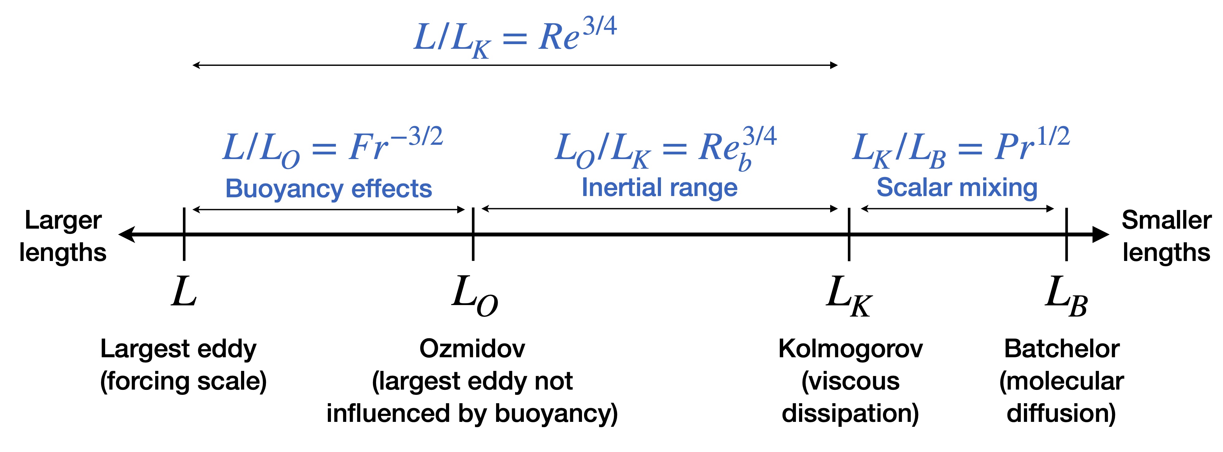
| $Re=\frac{UL}{\nu}$ | Controls separation between largest and smallest length scales in flow, with $L_B$ then controlling scales below $L_K$; $L/L_{K}=Re^{\frac{3}{4}}$ (assuming $\epsilon=U^{3}/L$) |
| $Fr=\frac{U}{LN}$ | Influence of stratification. Controls length scales influenced by buoyancy; $L_{O}/L=Fr^{\frac{3}{2}}$ |
| $Re_b = \epsilon / (\nu N^2)$ | Reynolds buoyancy number. Controls extent of inertial range uninfluenced by buoyancy; $L_{O}/L_{K}=Re_{b}^{\frac{3}{4}}$. Note $Re_{b}=ReFr^{2}$ assuming $\epsilon=U^{3}/L$ |
| $Pr=\frac{\nu}{\kappa}$ | Prandtl number. Controls separation between dissipation scales of velocity and density fluctuations; $L_{K}/L_{B}=\sqrt{Pr}$ |
The figure below illustrates the range of relevant length scales that must be resolved in a DNS of stratified turbulence.
Data formatting
Simulation outputs are stored as binary files of the form “{var}.{#}”, where {var}={u,v,w,r} corresponds to the three velocity components $(u,v,w)$ and the perturbed density field $\rho’$ away from the background density gradient. The {#} corrsponds to the timestamp of the simulation, which may be converted into a physical time based on the reported timestep.
The three-dimensional grid for a given variable and timestep is stored as a one-dimensional string of single-precision numbers in order of $x$ (fastest changing index), $y$, $z$ (slowest changing index). To easily detect errors in reading and reshaping the raw data into a three-dimensional grid, two zeros are padded onto the end of the $x$-dimension. The datafiles thus have size $\left(N_{x}+2\right)\times N_{y}\times N_{z}$. Python codes are provided to read and save a given binary file as a three-dimensional array (e.g. as a NumPy array). For larger datasets, it is advisable to use a memory map which allows one to easily extract slices of the fields without loading the entire three-dimensional array into memory.
Types of flows
DNS runs may be broadly categorized as follows, with further details and download links (if available) provided in the following tables:
- Time-independent (statistically-stationary) – A single snapshot of the steady turbulent flow (dissipation balanced by forcing) is provided for a given set of parameters. Turbulence is maintained via the following body forcing schemes:
- A. Forced no shear: Large spectral modes forced, without introducing mean shear, so as to maintain prescribed energy spectrum at large scales. Facilitates access to broad range of parameter space using relatively modest domains, particularly the high $Re_b$, low $Fr$ regime.
- Methodology: Almalkie and de Bruyn Kops, JoT, 2012
- B. Forced vertical shear: Background vertical shear injects energy; Richardson number $Ri$ varied to maintain fixed kinetic energy. Comparatively high $Fr$ relative to the other datasets.
- Methodology: Portwood, de Bruyn Kops, and Caulfield, PRL, 2019
- Methodology: Portwood, de Bruyn Kops, and Caulfield, PRL, 2019
- A. Forced no shear: Large spectral modes forced, without introducing mean shear, so as to maintain prescribed energy spectrum at large scales. Facilitates access to broad range of parameter space using relatively modest domains, particularly the high $Re_b$, low $Fr$ regime.
- Time-dependent evolution. Turbulence initialized using initial flow fields described below, then allowed to freely evolve without forcing. Multiple flow snapshots saved over time.
- C. Decaying: Field of unstratified turbulence generated, gravitational force is then introduced, flow is observed over time as it decays. Superior resolution of vast range of length-scales in limited region of $Re_b$-$Fr$ parameter space.
- Methodology: de Bruyn Kops and Riley, JFM, 2018
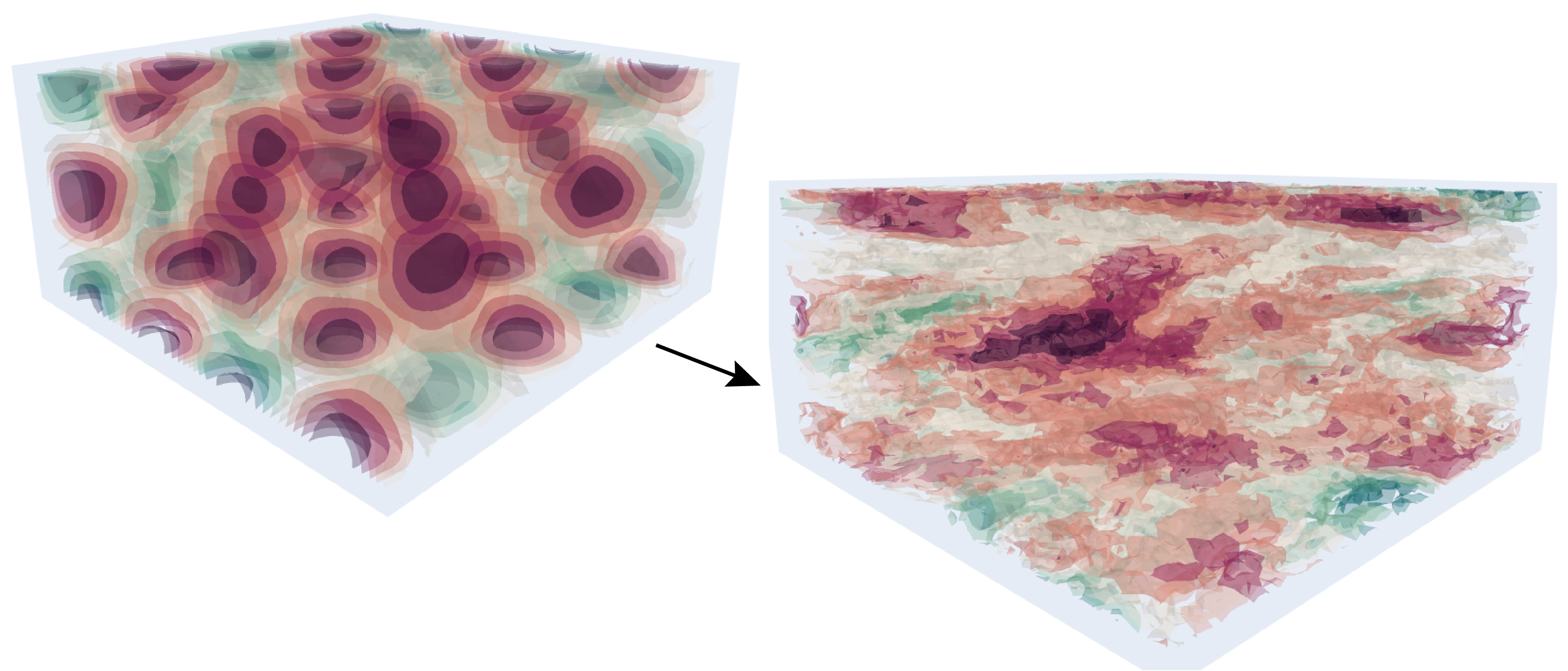
- D. Taylor-green vortices: Turbulence triggered by initially laminar field of Taylor-green vortices, develops, and then decays back to laminar state.
- Methodology: Riley and de Bruyn Kops, PoF, 2003
- C. Decaying: Field of unstratified turbulence generated, gravitational force is then introduced, flow is observed over time as it decays. Superior resolution of vast range of length-scales in limited region of $Re_b$-$Fr$ parameter space.
Taylor-green
- Three datasets spanning $Pr=\nu/\kappa=\left[1,7,50\right]$
- Fixed $Fr=2\pi U/\left(NL\right)=4$, $Re=UL/\nu=3200$
| Name, dataset link, parameter file | $Pr$ | Number of snapshots in time | Grid points $(N_x=N_y, N_z)$ | Field size (per variable, snapshot) | Total dataset size |
|---|---|---|---|---|---|
| TG_P1F4R32 | 1 | 15,000 | $512^2 \times 256$ | 255 MB | 15 TB |
| TG_P7F4R32 | 7 | 15,250 | $1280^2 \times 640$ | 4 GB | 244 TB |
| TG_P50F4R32 | 50 | 1,680 | $3584^2 \times 1792$ | 86 GB | 577 TB |
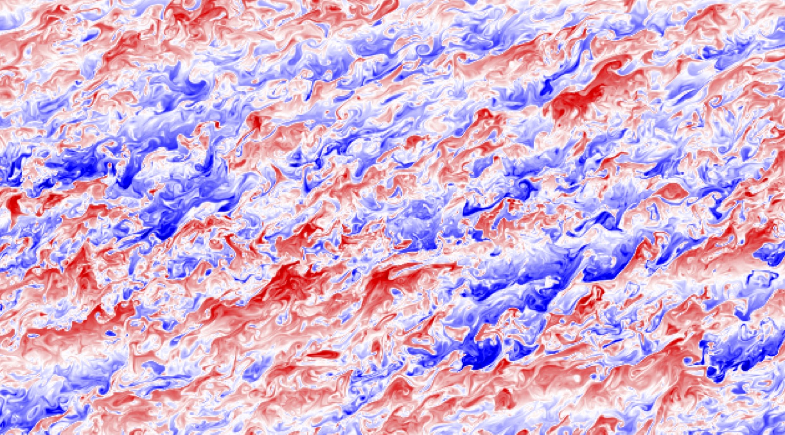
Forced vertical shear
- Fifteen datasets spannin three $Pr=\nu/\kappa=\left[1,7,50\right]$ and five buoyancy Reynolds numbers $(Re_b)=[30,1000]$
- Fixed Richardson number $Ri\approx 0.15$
Data upload expected to be complete by August 2026.
| Name and dataset link | $Pr$ | $Gn$ | Grid points $(N_x, N_y, N_z)$ | Field size (per variable, snapshot) |
|---|---|---|---|---|
| R1P1 | 1 | 34.7 | $1536 \times 768 \times 384$ | 1.7 GB |
| R1P7 | 7 | 34.0 | $3072 \times 1536 \times 768$ | 13 GB |
| R1P50 | 50 | 35.7 | $8000 \times 4000 \times 2000$ | 233 GB |
| R4P1 | 1 | 81.3 | $2048 \times 1024 \times 512$ | 3.8 GB |
| R4P7 | 7 | 83.1 | $5120 \times 2560 \times 1280$ | 62 GB |
| R4P50 | 50 | 84.0 | $16000 \times 8000 \times 4000$ | 1.87 TB |
| R6P1 | 1 | 213 | $3072 \times 1536 \times 768$ | 13 GB |
| R6P7 | 7 | 202 | $12288 \times 6144 \times 3072$ | 0.85 TB |
| R6P50 | 50 | 217 | $24000 \times 12000 \times 6000$ | 6.2 TB |
| R8P1 | 1 | 516 | $8736 \times 4368 \times 2184$ | 0.30 TB |
| R8P7 | 7 | 525 | $23040 \times 11520 \times 5760$ | 5.5 TB |
| R10P1 | 1 | 1026 | $12288 \times 6144 \times 3072$ | 0.85 TB |
| R10P7 | 7 | 813 | $31680 \times 15840 \times 7920$ | 14.5 TB |
Forced no shear
- Various datasets spanning $Pr=\nu/\kappa$,$Fr=2\pi U/\left(NL\right)$ and $Gn$

Data not currently uploaded to Constellation. Please contact group for access.
| Name | $Pr$ | $Fr_h$ | $Gn$ | Grid points $(N_x=N_y, N_z)$ | Field size (per variable, snapshot) |
|---|---|---|---|---|---|
| Pr = 1 | |||||
| P1F025Gn0014 | 1 | 0.039 | 14 | $14784 \times 14784 \times 1840$ | 1.61 TB |
| P1F035Gn0014 | 1 | 0.056 | 16 | $6144 \times 6144 \times 768$ | 116 GB |
| P1F050Gn0014 | 1 | 0.086 | 16 | $2048 \times 2048 \times 256$ | 4.3 GB |
| P1F070Gn0014 | 1 | 0.124 | 12 | $2048 \times 2048 \times 256$ | 4.3 GB |
| P1F100Gn0014 | 1 | 0.155 | 15 | $2048 \times 2048 \times 512$ | 8.6 GB |
| P1F150Gn0014 | 1 | 0.257 | 15 | $1024 \times 1024 \times 512$ | 2.1 GB |
| P1F200Gn0014 | 1 | 0.335 | 16 | $512 \times 512 \times 256$ | 268 MB |
| P1F300Gn0014 | 1 | 0.449 | 15 | $512 \times 512 \times 512$ | 537 MB |
| P1F400Gn0014 | 1 | 0.556 | 15 | $256 \times 256 \times 256$ | 67 MB |
| P1F500Gn0014 | 1 | 0.713 | 14 | $128 \times 128 \times 128$ | 8.4 MB |
| P1F025Gn0050 | 1 | 0.027 | 45 | $18432 \times 18432 \times 2304$ | 3.13 TB |
| P1F050Gn0050 | 1 | 0.070 | 53 | $8192 \times 8192 \times 1024$ | 275 GB |
| P1F100Gn0050 | 1 | 0.142 | 65 | $4096 \times 4096 \times 1024$ | 68.7 GB |
| P1F200Gn0050 | 1 | 0.334 | 45 | $2048 \times 2048 \times 1024$ | 17.2 GB |
| P1F400Gn0050 | 1 | 0.607 | 44 | $512 \times 512 \times 512$ | 537 MB |
| P1F600Gn0050 | 1 | 0.870 | 51 | $256 \times 256 \times 256$ | 67 MB |
| P1F800Gn0050 | 1 | 1.294 | 50 | $128 \times 128 \times 128$ | 8.4 MB |
| P1F025Gn0200 | 1 | 0.041 | 207 | $16384 \times 16384 \times 2048$ | 2.20 TB |
| P1F050Gn0200 | 1 | 0.105 | 194 | $14784 \times 14784 \times 1848$ | 1.62 TB |
| P1F100Gn0200 | 1 | 0.209 | 202 | $16384 \times 16384 \times 4096$ | 4.40 TB |
| P1F200Gn0200 | 1 | 0.322 | 207 | $4096 \times 4096 \times 2048$ | 137 GB |
| P1F400Gn0200 | 1 | 0.648 | 202 | $512 \times 512 \times 512$ | 537 MB |
| P1F800Gn0200 | 1 | 1.438 | 197 | $512 \times 512 \times 512$ | 537 MB |
| P1F1600Gn0200 | 1 | 2.578 | 206 | $256 \times 256 \times 256$ | 67 MB |
| P1F025Gn1000 | 1 | 0.026 | 1278 | $15840 \times 15840 \times 1980$ | 1.99 TB |
| P1F100Gn1000 | 1 | 0.210 | 1185 | $14784 \times 14784 \times 3696$ | 3.23 TB |
| P1F200Gn1000 | 1 | 0.419 | 1368 | $14784 \times 14784 \times 7392$ | 6.46 TB |
| P1F400Gn1000 | 1 | 0.564 | 929 | $3072 \times 3072 \times 3072$ | 116 GB |
| P1F800Gn1000 | 1 | 2.078 | 1044 | $1024 \times 1024 \times 1024$ | 4.3 GB |
| P1F1600Gn1000 | 1 | 3.619 | 1066 | $512 \times 512 \times 512$ | 537 MB |
| Pr = 7 | |||||
| P7F050Gn0050 | 7 | 0.078 | 57 | $30240^2 \times 3780$ | 13.8 TB |
| P7F100Gn0050 | 7 | 0.156 | 54 | $8192^2 \times 2048$ | 550 GB |
| P7F200Gn0050 | 7 | 0.289 | 64 | $6144^2 \times 3072$ | 464 GB |
| Pr = 50 | |||||
| P50F050Gn0050 | 50 | 0.073 | 54 | $37632^2 \times 4704$ | 26.6 TB |
| P50F100Gn0050 | 50 | 0.164 | 47 | $28672^2 \times 7168$ | 23.6 TB |
| P50F200Gn0050 | 50 | 0.315 | 66 | $8192^2 \times 4096$ | 1.1 TB |